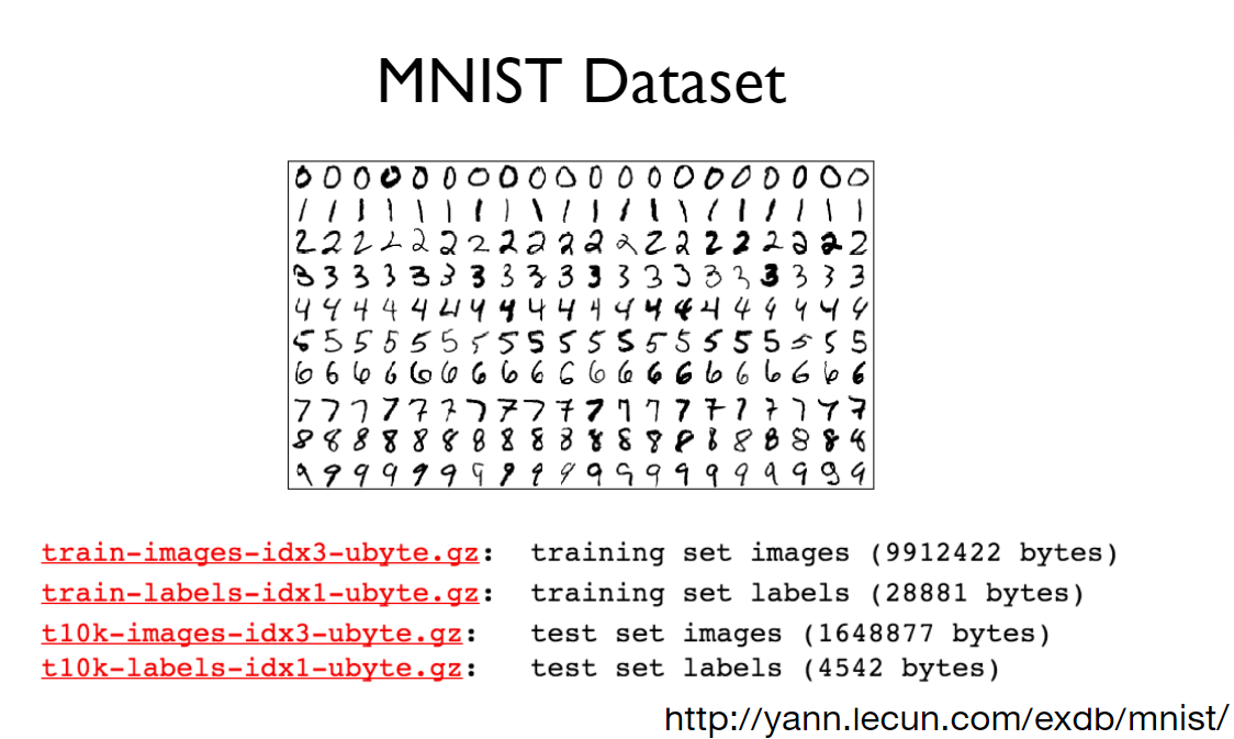
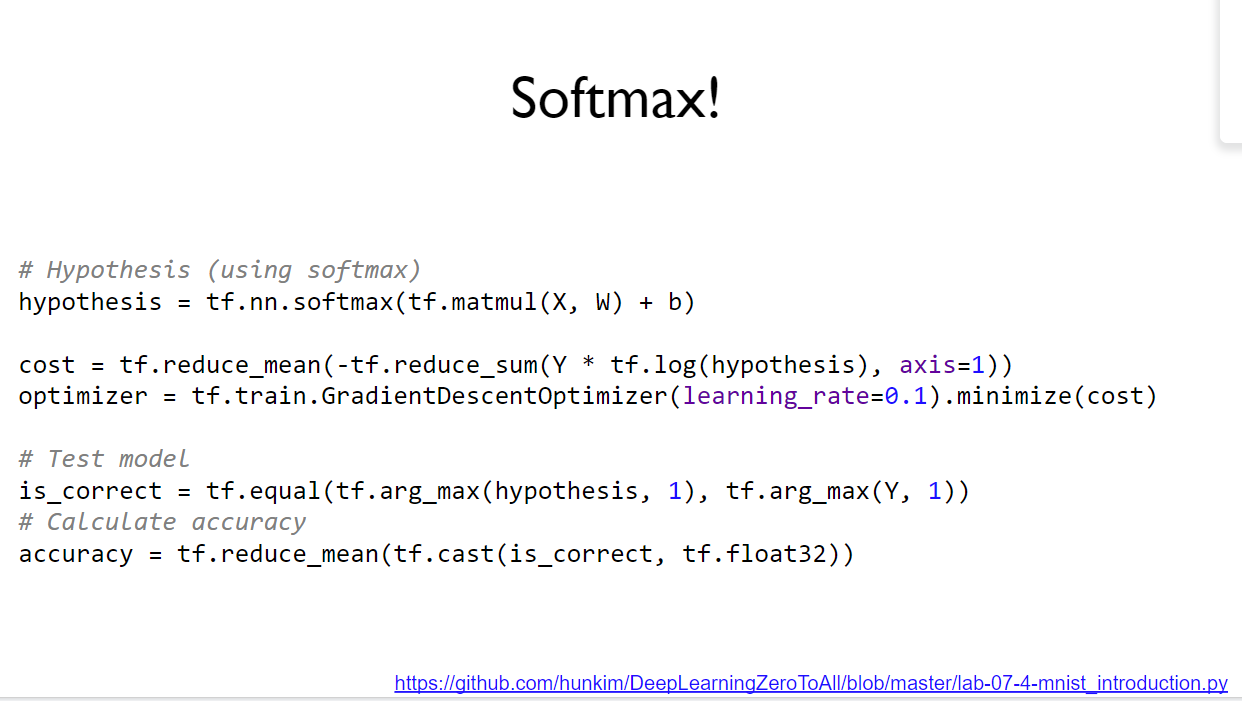
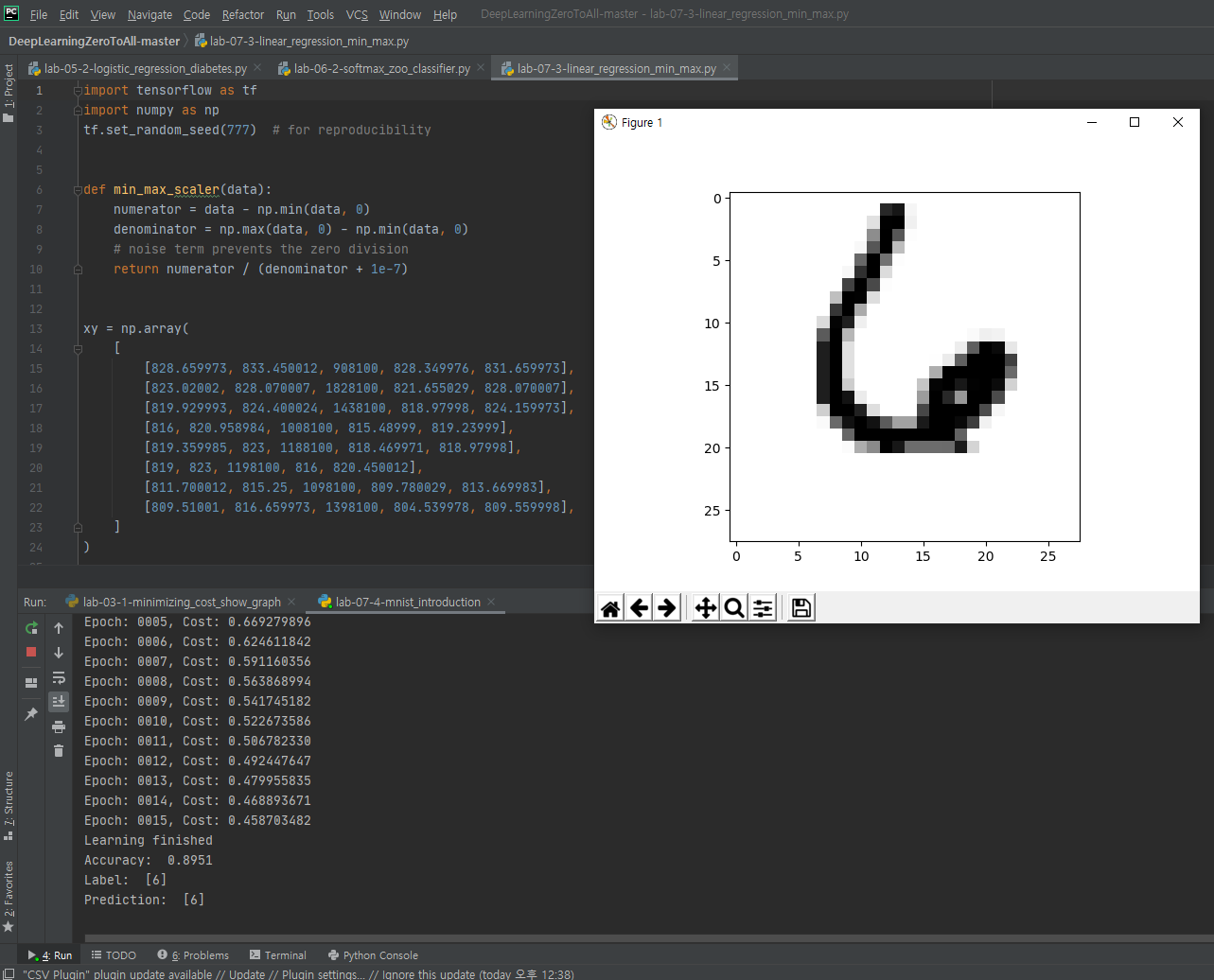
MNIST Dataset -손글씨 데이터-Tensoflow-cpu

본 샘플은 기본 과정을 다이해 했을때 소스의 구조를 이해 하게되는 예제 이다.

 

 

 

Training epoch/batch

 

In the neural network terminology:

• one epoch = one forward pass and one backward pass of all the training examples

• batch size = the number of training examples in one forward/backward pass. The higher the batch size, the more memory space you'll need.

• number of iterations = number of passes, each pass using [batch size] number of examples. To be clear, one pass = one forward pass + one backward pass (we do not count the forward pass and backward pass as two different passes).

Example: if you have 1000 training examples, and your batch size is 500, then it will take 2 iterations to complete 1 epoch.

---

코드

import tensorflow as tf
import numpy as np
tf.set_random_seed(777)  # for reproducibility


def min_max_scaler(data):
    numerator = data - np.min(data, 0)
    denominator = np.max(data, 0) - np.min(data, 0)
    # noise term prevents the zero division
    return numerator / (denominator + 1e-7)


xy = np.array(
    [
        [828.659973, 833.450012, 908100, 828.349976, 831.659973],
        [823.02002, 828.070007, 1828100, 821.655029, 828.070007],
        [819.929993, 824.400024, 1438100, 818.97998, 824.159973],
        [816, 820.958984, 1008100, 815.48999, 819.23999],
        [819.359985, 823, 1188100, 818.469971, 818.97998],
        [819, 823, 1198100, 816, 820.450012],
        [811.700012, 815.25, 1098100, 809.780029, 813.669983],
        [809.51001, 816.659973, 1398100, 804.539978, 809.559998],
    ]
)

# very important. It does not work without it.
xy = min_max_scaler(xy)
print(xy)

'''
[[0.99999999 0.99999999 0.         1.         1.        ]
 [0.70548491 0.70439552 1.         0.71881782 0.83755791]
 [0.54412549 0.50274824 0.57608696 0.606468   0.6606331 ]
 [0.33890353 0.31368023 0.10869565 0.45989134 0.43800918]
 [0.51436    0.42582389 0.30434783 0.58504805 0.42624401]
 [0.49556179 0.42582389 0.31521739 0.48131134 0.49276137]
 [0.11436064 0.         0.20652174 0.22007776 0.18597238]
 [0.         0.07747099 0.5326087  0.         0.        ]]
'''

x_data = xy[:, 0:-1]
y_data = xy[:, [-1]]

# placeholders for a tensor that will be always fed.
X = tf.placeholder(tf.float32, shape=[None, 4])
Y = tf.placeholder(tf.float32, shape=[None, 1])

W = tf.Variable(tf.random_normal([4, 1]), name='weight')
b = tf.Variable(tf.random_normal([1]), name='bias')

# Hypothesis
hypothesis = tf.matmul(X, W) + b

# Simplified cost/loss function
cost = tf.reduce_mean(tf.square(hypothesis - Y))

# Minimize
train = tf.train.GradientDescentOptimizer(learning_rate=1e-5).minimize(cost)

# Launch the graph in a session.
with tf.Session() as sess:
    # Initializes global variables in the graph.
    sess.run(tf.global_variables_initializer())

    for step in range(101):
        _, cost_val, hy_val = sess.run(
            [train, cost, hypothesis], feed_dict={X: x_data, Y: y_data}
        )
        print(step, "Cost: ", cost_val, "\nPrediction:\n", hy_val)

'''
0 Cost: 0.15230925 
Prediction:
 [[ 1.6346191 ]
 [ 0.06613699]
 [ 0.3500818 ]
 [ 0.6707252 ]
 [ 0.61130744]
 [ 0.61464405]
 [ 0.23171967]
 [-0.1372836 ]]
1 Cost: 0.15230872 
Prediction:
 [[ 1.634618  ]
 [ 0.06613836]
 [ 0.35008252]
 [ 0.670725  ]
 [ 0.6113076 ]
 [ 0.6146443 ]
 [ 0.23172   ]
 [-0.13728246]]
...
99 Cost: 0.1522546 
Prediction:
 [[ 1.6345041 ]
 [ 0.06627947]
 [ 0.35014683]
 [ 0.670706  ]
 [ 0.6113161 ]
 [ 0.61466044]
 [ 0.23175153]
 [-0.13716647]]
100 Cost: 0.15225402 
Prediction:
 [[ 1.6345029 ]
 [ 0.06628093]
 [ 0.35014752]
 [ 0.67070574]
 [ 0.61131614]
 [ 0.6146606 ]
 [ 0.23175186]
 [-0.13716528]]
'''

---

데이터 출처: http://yann.lecun.com/exdb/mnist/

MNIST handwritten digit database, Yann LeCun, Corinna Cortes and Chris Burges

소스설명: https://www.youtube.com/watch?v=ktd5yrki_KA&feature=youtu.be